A Sweeping Tour of TensorFlow

Over the past few months, I’ve been frequently switching between machine learning research projects and low-level infrastructure environments. Even though I’ve done a fair bit of work with TensorFlow, it always takes a non-zero amount of time to re-familiarize myself with TensorFlow’s API after I come back from building distributed systems in C++ for a few months. While first discovering TensorFlow, I wrote a bunch of notes about its basic API. I still find these notes a very useful ten minute read to reactivate the neurons in my brain responsible for TensorFlow, so I wanted to share them here without much modification. Don’t see this as a tutorial, but more of a quick overview or reference.

If you are more interested in TensorFlow’s architecture and design decisions, I wrote a technical report on that last year, which has become quite popular on the interwebs as it’s easier to digest than the official publication.

Graphs

TensorFlow represents computations as data flow graphs, composed of graph elements. A graph element may be a variable, a constant or an operation, representing some function of zero or more inputs. Moreover, tensor objects represent data flowing between graph elements, such as from one operation (e.g. a matrix multiplication) to another (e.g. a softmax function).

Graphs are objects in Tensorflow and can explicitly be created with a call to the Graph constructor. However, one cannot actually add elements to a graph directly. Rather, there is always a global default graph. All TensorFlow functions creating graph elements, such as Variable() or constant() operate on this default graph. Upon startup of the library, there already exists a default graph, so you can create a computational graph without constructing a new Graph. If you do want to maintain multiple graphs, you’ll have to set the specific Graph to be the current default graph via the graph.as_default() context manager:

import tensorflow as tf

# Create a new graph
graph = tf.Graph()

with graph.as_default():
	...

Later, you can choose which graph to execute by passing the respective graph to the tf.Session() constructor (as graph=<graph>):

graph = tf.Graph()
with graph.as_default():
	v = tf.Variable(tf.random_uniform(shape=[2, 2], dtype=tf.float32))
	y = tf.nn.relu(v)

with tf.Session(graph=graph) as session:
	tf.initialize_all_variables().run()
	print(session.run(y))

Tensors

In TensorFlow, any data flowing between two nodes in the computational graph is represented by a tensor. A tensor is an $n$-dimensional collection of homogenous values with a fixed, static type. The number of dimensions a tensor has is described by its rank. For example, a tensor with rank 1 is a vector, while a rank-2 tensor would commonly be known as a matrix. Given a rank $r$, a tensor is additionally associated with a shape. The shape of a tensor is a vector of size $r$, specifying the number of components the tensor has for each of its $r$ dimensions. It is important to note that even scalars or strings are tensors. In this case, they simply have a rank of zero.

In terms of the computational graph, a tensor represents a symbolic handle to one of the outputs of an Operation. It does not hold the values of that operation’s output, but instead provides a means of computing those values in a TensorFlow Session.

Data types

A tensor can have any of the following types:

• tf.float32: 32-bit float
• tf.float64: 64-bit float
• tf.int8: 8-bit signed integer
• tf.int16: 16-bit signed integer
• tf.int32: 32-bit signed integer
• tf.int64: 64-bit signed integer
• tf.uint8: 8-bit unsigned integer
• tf.string: variable-length string
• tf.bool: Boolean truth value
• tf.complex64: 64-bit complex value composed of 32-bit real and imaginary part

Constants

The simplest kinds of computational units in a TensorFlow graph are constants, representing some value that will not change during evaluation of the graph. This is always a tensor, from zero-dimensional scalars or strings to higher dimensional tensors.

TensorFlow provides a rich API for creating constants. The simplest way is tf.constant(value, dtype, shape, name), which takes a value as well as an optional datatype, shape and name. The value can either be a constant value (i.e. a Python number, string etc.) or a list of homogenous values. If shape is specified but the value’s shape does not match, the last (and possibly only) value of value will be used to fill the tensor across all dimensions to statisfy the requested shape:

with tf.Session():
	# 5
	print(tf.constant(5).eval())
	# 'Hello, World!'
	print(tf.constant('Hello, World!').eval())
	# [[5, 5], [5, 5]]
	print(tf.constant(5, shape=[2, 2]).eval())
	# [[1, 2, 2], [2, 2, 2], [2, 2, 2]]
	print(tf.constant([1, 2], shape=[3, 3]).eval())

There exist various other ways of creating constants, such as:

• tf.zeros(shape, dtype, name): Creates a tensor of zeros.
• tf.ones(shape, dtype, name): Creates a tensor of ones.

• tf.ones_like(tensor, dtype, name): Creates a tensor of zeros with the same shape as another tensor.

• tf.linspace(start, stop, num): Creates a vector of num values, starting at start and ending at stop.
• tf.range(start, limit, delta): Same semantics as the Python range function.

Variables

Variables maintain state in the graph that can be updated by the computational graph during evaluation or by the user directly. More precisely, variables are in-memory buffers containing tensors.

When creating a variable, you must pass it some initial tensor of some shape or type, which then defines the shape and type of the variable. You can later change the value of the variable with one of the tf.assign functions provided by TensorFlow. While the data type remains fixed, you can also modify the shape of the variable by setting the validate_shape flag to False when assigning a new value.

It is important to note that the variable does not actually store the initial value. Rather, when constructing a Variable with some value, the following three graph elements are added to the current default graph:

1. A variable element that holds the variable value.
2. An initializer operation that sets the initial value to the variable, i.e. a tf.assign node.
3. A node to hold the initial value, such as a tf.constant node.

When you launch your graph, you first need to initialize the variables you created. That is, you must evaluate all the initialization operations (2) to assign the initial tensors (constants) to the variables. You could do this explicitly for each variable by accessing the variable’s initializer attribute:

v = tf.Variable(tf.constant(5))
with tf.Session() as session:
	session.run(v.initializer)

However, the more common idiom is to add a node to the graph that evaluates all the initializers of all the nodes. You do this by calling tf.global_variables_initializer():

with tf.Session() as session:
	tf.global_variables_initializer.run()

Any variable you add to your current default graph is added to its collection of variables, which you can retrieve via tf.all_variables(). Note that the Variable constructor also has a parameter trainable=<bool>, which determines whether to add the variable to the graph’s list of trainable_variables. This is the list consulted by the Optimizer class to determine which variables to train during optimization. The trainable parameter defaults to True.

As stated above, a variable does not actually hold any (valid) value until its initializer was evaluated. If you nevertheless wish to create a variable using the (initialized) value of another variable, you can use the variable.initialized_value() function to retrieve a tensor that can be used to initialize another variable:

w = tf.Variable(tf.random_normal(shape=[5, 5], stddev=0.5))
v = tf.Variable(w.initialized_value())
u = tf.Variable(v.initialized_value() * 2.0)

If you want to give a variable a new value, you can use one of the following functions (there are more):

1. Variable.assign(value): Assign a new value.
2. Variable.assign_add(delta): Add a value to the variable.
3. Variable.assign_sub(delta): Subtract a value from the variable.

Note that for each of these member functions (methods), there exists an equivalent non-member function in the tf namespace (e.g. tf.assign(tensor, value)).

Placeholders

A placeholder is a graph element representing a tensor whose values must be supplied at the start of graph-evaluation. It is constructed with a given data type and shape and must always be fed when calling Session.run() or Tensor.eval(). More precisely, when calling one of these functions, you can supply a feed_dict parameter that is a dictionary mapping any placeholders in the graph to some values that match their data type and shape. If you do not pass a value for any of the placeholders, the tensor will produce an error upon attempted evaluation. Note also that the shape of the value supplied is checked against the shape specified for the place-holder.

x = tf.placeholder(dtype=tf.float32, shape=[2, 2])
y = tf.matmul(x, x)

with tf.Session() as session:
	session.run(y) # will fail!
	session.run(y, feed_dict={x: [[1, 2], [3, 4]]}) # OK

Operations

Operations tie together computational nodes in the graph. Such an operation can take zero or more tensors as input and produce zero or more tensors as output. The following shows the use of a simple operation:

a = tf.Variable(tf.constant(5, shape=[2, 2], dtype=tf.float32))
b = tf.Variable(tf.random_uniform(shape=[2, 2]))

c = a + b

with tf.Session() as session:
	session.run(tf.initialize_all_variables())
	print(c.eval())

Note that all nodes are really operations. A constant is an operation that takes no inputs and always produces the same tensor. A Variable is an operation that returns a handle to a mutable tensor that may be updated by special assign operations.

Sessions

In TensorFlow, operations are executed and tensors are evaluated only in a special environment referred to as a session. Inside such a session, resources such as variables, queues or readers (for reading data from disk) are allocated. Naturally, these resources must also be freed again later on. For this reason, there are two parallel APIs for Session objects:

1. Create the Session object manually and close it yourself,
2. Use a context manager for the entire duration of the session.

In the first case, you have more control over the lifetime of the session. You can create one with session = tf.Session(graph=graph), then run operations or evaluate tensors with session.run(fetches). At the end, you need to call session.close() to release any resources. In between, you can also make the session the default session (such that you can call run on operations and eval on tensors) by using the session.as_default() context manager:

session = tf.Session(graph=graph)

with session.as_default():
	op.run()
	tensor.eval()

Note that this does not close the session. You can also use the session object itself as a context manager, but then the session will be closed when leaving the scope:

with session:
	op.run()
	tensor.eval()

This is really also the essence of the “second API”: just create a session with tf.Session(graph=graph) and use it directly as a context-manager:

with tf.Session(graph=graph) as session:
	op.run()
	tensor.eval()

This way, you’ll never need to remember to close the session yourself. Note that tensor.eval() and operation.run() both also take an optional Session argument, if you want to run just a single operation or evaluate a single tensor without a full context manager.

feed_dict

Session.run() additionally accepts an optional feed_dict, that was already discussed for placeholders. Note, however, that this dictionary can not only contain placeholder tensors, but any tensor in the graph that should be substituted with a concrete value:

a = tf.constant(5)
b = a + 10

with tf.Session() as session:
	print(session.run(b)) # 15
	print(session.run(b, feed_dict={a: 10})) # 20

This is similar to Theano’s givens parameter to theano.function.

InteractiveSession

There additionally exists the InteractiveSession class, which, when constructed, registers itself as the default session. Therefore, when you are in a shell for example, you can just create one such interactive session and run()/eval() your operations and tensors without a context-manager or needing to pass a session to run() or eval(). However, you need to close() the session to free resources at the end:

session = tf.InteractiveSession()
a = tf.constant(5)
b = tf.constant(6)
c = a + b
print(c.eval())
session.close()

Control Dependencies

Most edges in the computational graph are data flow edges, through which tensors flow. However, there exists another class of edges called control dependencies. A control-dependency from node $A$ to node $B$ specifies that $A$ must have finished executing before $B$ is allowed to execute. This can be used to synchronize the data flow.

In code, TensorFlow’s Graph class provides the control_dependencies() function. This method takes a list of tensors or operations and returns a context-manager. When called in with-as statement, all operations and tensors defined in the context (scope) of the statement will have control-dependencies on all nodes in the list passed to the function:

graph = tf.Graph()
a = ...
b = ...
with graph.control_dependencies([a, b]):
	c = ...
	d = ...

Here, nodes c and d will have control-dependencies on both a and b. This means that during execution, node c will only be evaluated once a and b have been evaluated. You can also just use tf.control_dependencies() instead of the Graph member function, to implicitly use the default graph.

Control Flow

There exists a variety of possibilities to adjust control flow in the computational graph.

If-Statements

The simplest such possibility is to return one or the other tensor depending on some boolean condition, i.e. an if-statement in a conventional programming language. For this, one can use tf.cond(condition, if_so, else) or tf.case(condition_callable_pairs), which emulates a switch-case statement. In the first case, condition is a boolean scalar (i.e. 0-dimensional tensor), while the other two parameters are callables that return tensors. Both functions must return lists (or single) output tensors and must return the same number of outputs in any case:

a = tf.constant([1, 2, 3])
b = tf.constant([4, 5, 6])
x = tf.placeholder(shape=[], dtype=tf.bool)

c = tf.cond(x, lambda: a, lambda: b)

with tf.Session() as session:
    # [1, 2, 3]
	session.run(c, feed_dict={x: True})
	# [4, 5, 6]
	session.run(c, feed_dict={x: True})

The case method takes a list of (boolean, callable) pairs as well as a callable default. Thirdly, an optional boolean exclusive may be supplied. If exclusive is false, the function will check each pair in order until the first condition yields true. It then returns immediately without evaluating the other conditions. If no condition is true, the result of the default callable is returned. If exclusive is set to true, all predicates are evaluated and if more than one yields true, an error is raised. If no condition is true, the result of default is returned once more:

a = tf.constant([1, 2, 3])
b = tf.constant([4, 5, 6])
x = tf.placeholder(shape=[], dtype=tf.int32)

c = tf.case([(x > 5, lambda: a), (x < 5, lambda: b)], lambda: tf.constant(-1))

with tf.Session() as session:
	# [1, 2, 3]
	session.run(c, feed_dict={x: 10})
	# [4, 5, 6]
	session.run(c, feed_dict={x: 3})
	# [-1]
	session.run(c, feed_dict={x: 5})

While Loops

while-loop and for-loops are both expressed via the while_loop function. Its arguments are a callable cond taking a list of tensors and returning a truth value; a callable body taking the same list of tensors and returning a new list of tensors of same shapes and types as well as a list of tensors loop_vars to pass to cond and body:

i = tf.constant(0)
loop = tf.while_loop(lambda i: i < 10, lambda i: i + 1, [i])

with tf.Session():
	# 10
	print(loop.eval())

def body(x):
	a = tf.constant(tf.random_uniform(shape=[2, 2], dtype=tf.int32, maxval=100))
	b = tf.constant(np.array([[1, 2], [3, 4]]))
	c = a + b
	return tf.nn.relu(x + c)

def condition(x):
	return tf.reduce_sum(x) < 100

x = tf.Variable(tf.constant(0, shape=[2, 2]))

with tf.Session():
	tf.initialize_all_variables().run()
	result = tf.while_loop(condition, body, [x])
	print(result.eval())

The operation returns the list of tensors that invalidated the condition.

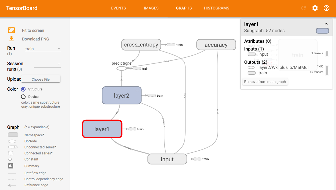
Visualization

TensorFlow comes with an extremely useful and powerful visualization tool called TensorBoard, with which you can view and explore your neural network architecture in an interactive fashion, track histograms and value distributions of weights, visualize convolution kernels, record speech samples and more.

Values you wish to visualize in TensorBoard are tracked using summary nodes. A summary node is an operation embedded in the data flow graph that will write information about particular values of interest in your graph to a predefined directory, in a format understood by the TensorBoard server. There are two main kinds of summaries: scalar summaries (tf.summary.scalar) and histogram summaries (tf.summary.histogram). The former track values and get displayed in a two-dimensional plot over time, while the latter produce graphs visualizing the distribution of values over time (for example the distribution of weights of a particular layer in your CNN). For example:

x = tf.Variable(1.0)
y = tf.Variable(2.0)
# Will display the value of x + y over time
tf.summary.scalar('z', x + y)

w = tf.Variable(tf.random_normal(shape=[32, 32], stddev=0.1))
# Will display the distribution of values in w over time
tf.summary.histogram('w', w)

You can (and probably should) namespace nodes, using tf.name_scope. This is useful when you have multiple layers for example. You can call all your weights w but have them in different namespaces, e.g. conv1/w and conv2/w:

with tf.name_scope('conv1'):
  w_conv1 = tf.Variable(...)
  tf.summary.scalar('w', w) # will show up as 'conv1/w'

To write summaries to disk for TensorBoard to pick up, you use a tf.summary.FileWriter and initialize it with the path to dump data to and the graph to display (usually from your session):

with tf.Session() as session:
  writer = tf.summary.FileWriter('/tmp/log', graph=session.graph)

Then, you’ll usually want to merge all summaries into one operation, as well as have a global step variable to track your epochs. Finally, you can have code like this to write a summary after every training step:

merged = tf.summary.merge_all()
with tf.Session() as session:
    writer = tf.summary.FileWriter('/tmp/log', graph=session.graph)
    for step in range(1000):
        writer.add_summary(merged.eval(), global_step=step)

While training your model, you can then start a TensorBoard server:

$ tensorboard --logdir=/tmp/log