I recently presented the paper Dremel: Interactive Analysis of Web-Scale Datasets by Melnik et al. (2010) in my team’s paper reading group at work. The paper presents one of Google’s foundational data analysis systems and is an interesting read for anyone interested in the intersection of data analytics, database systems and distributed systems. In particular, it is enlightening to understand the design decisions required to make this system operate at the scale of petabyte-sized datasets – inevitably many datasets at Google’s scale.
The purpose of this blog post is to provide a walkthrough of the paper in alternative wording, which may be useful to you if you have read the paper and are seeking clarification on certain points; or simply prefer the language of a blog over that of an academic paper. That said, the paper is itself a relatively easy read and I encourage you to review the original paper before or after reading this post.
TL;DR
For the busy executives among you, I like to provide a quick TL;DR summary:
Dremel is Google’s internal data analysis and exploration system. It is designed for interactive (i.e. fast) analysis of read-only nested data. Its design builds on ideas from parallel database management systems as well as web search.
The key contributions of the paper are:
- A column-striped storage format for nested data,
- A SQL-like language adapted to nested data,
- Use of execution trees from web search systems applied to database queries.
Overall, the paper shows that it is possible to build a system that enables analysis of trillions of read-only records spanning petabytes of storage at interactive speeds usually below 10 seconds. If you want to learn more about how, read on.
Motivation
Let’s begin by understanding the motivation for building Dremel. The observation the Dremel paper makes in its introduction is that data found in typical “web computing” environments is often non-relational. Non-relational here means that it is not natural to fit the data exchanged by such web computing systems into a relational model, i.e. a flat collection of tuples as you would store them in your run-of-the-mill MySQL database. Typical examples of such non-relational data include:
- Messages exchanged by distributed systems (think: Protocol Buffer messages or Thrift structs),
- Structured documents like websites,
- Data structures used in everyday programming languages.
Notice especially that each of these categories of data usually involve nested data. Further, the paper makes the observation that if you were to store such data using a relational model, the process of de-structuring, or “unnesting”, and re-structuring this data, as well as splitting it into well-normalized database tables, is prohibitive at web scale.
So, what if we could …
- Store such data in its original, nested structure,
- Access data as-is without re-structuring it,
- Describe queries on nested data without complicated joins
… and do all of this blazingly fast on petabytes of data for interactive analysis. Well, lo and behold, this is what Dremel was designed for!
Trivia
Before we dive into the nitty gritty details of how Dremel works, it may be entertaining to know some trivia about it first.
Dremel has been in production at Google since 2006. A selection of use cases for Dremel at Google include analysis of:
- Crawled web documents,
- Spam,
- Build system results and
- Crash reports.
Further, there are two ways to use Dremel outside of Google. The first is Google’s BigQuery service, which Google provides as part of its cloud offering. The second is Apache Drill, effectively an open source re-implementation of Dremel.
But wait, what about the name? Turns out, Dremel is a pretty clever name: “Dremel is a brand of power tools that primarily rely on their speed as opposed to torque”.
Technical Details
The next few paragraphs digest the technical details of the Dremel paper, roughly in their original order.
Data Model
Arguably the most important pillar of the Dremel system is that its data model centers around nested data. What is nested data? In essence, and likely in practice, this just means data that can be described with the Protocol Buffers specification. Protocol Buffers is Google’s data serialization format, and comes with an interface description language (IDF) that allows defining nested data structures. Here is an example of a nested data structure, a.k.a. record, defined in the Protocol Buffer IDF:
message Document {
  required int64 DocId;
  optional group Links {
    repeated int64 Backward;
    repeated int64 Forward; }
  repeated group Name {
    repeated group Language {
      required string Code;
      optional string Country; }
    optional string Url; }}
If you’ve never seen a Protocol Buffers record (or message) before, you should notice:
- It describes a nested data structure,
- Fields or sub-records (groups) can be:
- required (must be present),
- optional (can be omitted),
- repeated (occur zero or more times).
There is an important connection between optional and repeated fields in that both can be omitted. Omitted here means that it need not have a value when serializing a concrete object from some programming language into the final data format (which can then be stored or sent over the wire). This will become very relevant in the later discussion on lossless storage of such records.
A final piece of important nomenclature associated with nested data records is a field’s path. In the above record, each named entity is a field. The path to a field is the dot-separated list of fields one would traverse in order to reach that field. Examples of field paths are:
Document.Links.Forward,Document.Name,Document.DocId.
In the paper and this article, the top-most field name is often omitted, e.g.
Name.Language.Country is synonymous with Document.Name.Language.Country.
Storage Model
Given a data model, any data management system must decide how to store data following this model. This is called the storage model. For this, Dremel borrows from the world of Online Analytical Processing (OLAP) relational databases, which for many years now have exploited the benefits of column-oriented storage. The idea of column-oriented storage in the world of relational databases is very simple: Instead of storing tuples “row after row” in memory, data is stored “column after column”. For this table:
| A | B | C |
|---|---|---|
| 0 | 1 | 2 |
| 3 | 4 | 5 |
| 6 | 7 | 8 |
storing the data in this table in a row-oriented fashion would mean storing them in memory row-by-row:
Data:        0 | 1 | 2 $ 3 | 4 | 5 $ 6 | 7 | 8
Memory Cell: 0 | 1 | 2 | 3 | 4 | 5 | 6 | 7 | 8
where I use $ to denote row boundaries. In column-oriented layout, columns are
stored next to each other in memory:
Data:        0 | 3 | 6 $ 1 | 4 | 7 $ 2 | 5 | 8
Memory Cell: 0 | 1 | 2 | 3 | 4 | 5 | 6 | 7 | 8
where $ now indicates a column boundary. The latter layout is beneficial to
queries that do not read entire rows at a time, but access only specific
columns. It turns out that most data analysis workloads are like this. For
example, the following “business intelligence” analysis
SELECT SUM(price) from Purchases WHERE date > '2019-01-01'
looks at only two columns in a table with potentially hundreds of columns. In column-oriented storage, the DB engine can scan through only the columns it needs, while in row-oriented storage it (naively) would need to access the entire row (all columns).
Things are not quite the same for Dremel since its data model revolves around
nested data as opposed to flat, relational data. Nevertheless, Dremel is an
analytical query engine and wants to access individual fields quickly.
Therefore, one innovation Dremel makes is to employ a column-striped layout for
its storage model too, resulting in greater efficiency and fast encoding and
decoding of data. It is noteworthy to mention what column-oriented storage
actually means for nested data. Effectively, it means storing the “leaf”
fields side-by-side in memory just like the column values in the second example
above. In the record presented in the previous section, examples of leaf fields
would be Document.DocId or Document.Links.Backward. Note that group fields
like Document.Name aren’t stored themselves, since they exclusively influence
the logical structure of the data but do not store data themselves. Only a leaf
field can actually have a value.
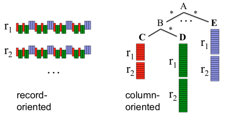
The figure below, taken from the paper, illustrates the difference between storing a record in record-oriented format, which you can think of as row-oriented, versus the column-oriented format that Dremel employs instead.
In terms of how columns are physically stored, the paper explains that a distributed file system such as the Google File System (GFS) is a suitable choice.
The next section discusses the challenges in implementing column-striped storage for nested data.
Lossless Columnar Representation
As the previous paragraph explained, Dremel uses column-oriented storage, which means leaf fields are stored contiguously in memory. Interestingly, this means that the values are “lifted” out of their logical structure. Take the following record:
Name
    Language:
        Code: 'en'
    Language:
        Code: 'en-us'
Name
    Language:
        Code: 'en-gb'
In a column-oriented storage model, values of the Name.Language.Code field
will be stored in memory like this:
'en'
'en-us'
'en-gb'
In the original record, each value had a logical location within the record
structure. However, now values are stored in an entirely flat manner. Upon
re-assembly, how do we know that the first two values belong to the first Name
group and the third value to the second Name group?
This is where the Dremel paper introduces two additional pieces of information that is stored with each field value to achieve lossless columnar representation. The first piece of information is called the repetition level and the second is termed the definition level.
Repetition Level
The repetition level tells us at what repeated field in a field’s path the
value has repeated. Recall that in our running record example, both Name and
Name.Language are repeated groups. As such, for a field path like
Name.Language.Code, the repetition value tells us whether a particular value
belongs to a repetition of the inner group Name.Language or to the outer group
Name. Consider our previous record:
Name:
    Language:
        Code: 'en'
    Language:
        Code: 'en-us'
Name:
    Language:
        Code: 'en-gb'
For the value en-us, it was the Language group that repeated “most recently”.
For the en-gb value, it was the entire Name group that repeated most
recently. As such, the repetition level of the latter value is 1, because in
the field path Name.Language.Code it is the first field, Name, that was
repeated. For the former example, en-us, the repetition value is 2, because it
is the second field, Name.Language, that repeated last. For the the very first
value in the record, en, the repetition level is 0 because it’s the Document
itself that repeated most recently (it didn’t actually “repeat” because it’s the
first record in this example, but alas, this is the base case).
Equipped with the power of assigning a repetition level to each value we store, we can go back and amend our in-memory layout from above to the following:
'en'    | 0
'en-us' | 2
'en-gb' | 1
Here I’ve written the repetition numbers in the right-most column.
Definition Level
Another number Dremel associates with each stored value is its definition
level. This level indicates how may fields in a path that could be omitted,
are actually present. In Name.Language.Code, both Name and Name.Language
are repeated groups, which means they could be omitted. If Name is however
present in a field’s path, the definition level is bumped to 1. If
Name.Language is present too, the definition level is bumped to 2. This number
becomes relevant for encoding of NULL values. In the following record:
Name:
    Language:
        Code: 'en-us'
        Country: 'USA'
    Language:
        Code: 'fr'
Name:
    Language:
        Code: 'en-gb'
        Country: 'USA'
The second Name.Language group has omitted the Name.Language.Country field.
This information has to be stored in form of a NULL value in the
Name.Language.Country column. What the definition level tells us, then, is how
much of the record surrounding a field is omitted. In the above record, the
Name and Name.Language group are present, but not the final
Name.Language.Country field. The definition level of that NULL value would
be 2, because it’s two ancestor fields are present in the record. In this record:
Name:
    Url: 'http://www.example.com'
the Language group is omitted as a whole, so the definition level of the
NULL value we store for the invisible Name.Language.Country field is 1.
Zooming out further:
Document:
    DocId: 1
Document:
    DocId: 2
this record doesn’t even have a Name group, so we’d store a NULL value for
the Name.Language.Country column with definition value 0, because none of the
optional or repeated fields in the path Name.Language.Country, which are
Name, Name.Language and Name.Language.Country, are present.
My understanding of the purpose of this value is not to aid in lossless storage.
This, as far as I can tell, is accompalished by the repetition level alone. I
believe the purpose of this number is to be able to store NULL values without
storing an actual value. That is, any definition level smaller than the length
of the path indicates that the value is NULL. The exact value then tells us
how much of the path is omitted. Many real-world datasets are very sparse (have
lots of NULL values), so efficient encoding of NULL values would have high
priority in a design for a system like this.
Storage of Repetition and Definition Level
The paper mentions a number of optimizations that are used to store definition
and repetition levels efficiently. One such optimization is to omit explicit
NULL values as the definition level already reveals whether a value is present
in the final record or not. Further, definition levels are not stored for
required fields, since by the nature of that qualification the field and thus
its whole path must be defined. Also, if the definition level is zero, the
repetition level must be zero too because the whole group (one level below the
whole record, e.g. Document) is omitted. Levels in general stored in a
bit-packed fashion.
Assembly of Records
As we’ll review in more detail later, Dremel emits records as its query output. To do so, it must assemble records from the data columns it reads from memory. What is particularly important and interesting about this task is that Dremel must be able to read partial records. That is, records that follow the structure of the record schema (the Protocol Buffer specification) while omitting certain fields or entire groups. The paper describes that at Google many datasets are sparse, often with thousands of fields in the record schema, of which usually only a small subset is queried.
Most of the examples we’ve looked at so far were partial records, for example in
Name:
    Language:
        Code: 'en-us'
the only field present is Name.Language.Code. Fields like
Name.Language.Country and entire groups such as Links are omitted.
Nevertheless, the record follows the original schema, with Language nested
under Name and Code under Language.
To do the actual record assembly, Dremel creates a Finite State Machine (FSM). Here is an example figure from the paper:

This FSM constructs the record by logically jumping from column to column and scanning values from memory until exhausted. Edge values indicate repetition levels.
Query Language
Now that we know more about how Dremel encodes and assembles records, let’s move on to investigate how Dremel allows users to query these records. For this, Dremel provides a SQL-like query language. Overall, the look and feel of this language is very much like SQL, with the noteable exception that fields can be referenced by their full, nested path. Here is an example query:
SELECT DocId AS Id,
  COUNT(Name.Language.Code) WITHIN Name AS Cnt,
  Name.Url + ',' + Name.Language.Code AS Str
FROM t
WHERE REGEXP(Name.Url, '^http') AND DocId < 20;
In general, this query language takes a table – a collection of records following one particular schema – as input and produces zero or more (partial) records as output. Note again: instead of rows, it outputs records. Here is an example of a single record emitted as output:
DocId: 10
Name:
    Cnt: 2
    Language:
        Str: 'http://A,en-us'
        Str: 'http://A,en'
Name:
    Cnt: 0
There are three important points to mention about this query language, which can all be observed in the query and its result. These are how Dremel deals with selection, projection and aggregation. The following paragraphs dive into these three aspects.
Selection
The first point is about how Dremel does selection. Selection is accomplished
via the usual WHERE statement. In the query above, it is the statement
WHERE REGEXP(Name.Url, '^http') AND DocId < 20;
For the nested record structures Dremel operates on, selection conceptually has
the semantics of “pruning subtrees”, as the paper puts it. The idea is that
given a record substructure, or subtree, the WHERE statement has the effect of
taking the entire tree out of consideration if it does not match the selection
predicate. Above, if a particular Name substructure of a Document record
does not have a Url field matching the '^http' regular expression, the whole
Name substructure is thrown away. This means its Name.Language.Code field,
albeit a different field from Name.Url, will not be used to produce a record
even though it is referenced in the projection (line 2 in the full query). The
second clause in the selection, DocId < 20, prunes away entire records, i.e.
Documents, at the top-most level.
Projection
Projections in Dremel have the interesting semantics that if a projection involves two fields at different levels of nesting, values will be produced for every field at the most-nested level. Consider the projection
Name.Url + ',' + Name.Language.Code AS Str
Here, Name.Url is at nesting level 2 (starting at Document), while
Name.Language.Code is nested one level more. This means there could be many
Name.Language.Code values for one Name.Url within a Name group. The
semantics of Dremel here dictate that one value will be produced for each value
at the most-nested level, i.e. one value for every Name.Language.Code, using
the same Name.Url. This is exemplified by the sample output shown above, which
could have been produced by a record like this (disregarding selection):
Name:
    Url: 'http://A'
    Language:
        Code: 'en'
    Language:
        Code: 'en-us'
Aggregation
Dremel’s aggregation semantics are showcased by the following line in the original query:
COUNT(Name.Language.Code) WITHIN Name AS Cnt
Make particular notice of the WITHIN keyword, which is not part of ANSI SQL
since ANSI SQL’s data model includes only flat data. Because Dremel operates on
nested data, it is necessary to specify at which level of nesting the
aggregation should be performed. Consider this record:
Name:
    Language:
        Code: 'en'
    Language:
        Code: 'en-us'
Name:
    Language:
        Code: 'en-gb'
Counting how many Name.Language.Code fields there are could mean different
things here. We could count how many such fields there are in the entire record
or we could count how many such fields there are within each Name group. This
is what the WITHIN keyword gives us control over. Above, we specify to
aggregate WITHIN Name, which means we’ll produce one Cnt value for each
Name group. This produces the output from above:
DocId: 10
Name:
    Cnt: 2
    Language:
        Str: 'http://A,en-us'
        Str: 'http://A,en'
Name:
    Cnt: 0
If we instead wrote
COUNT(Name.Language.Code) WITHIN Name.Language AS Cnt
we would get
DocId: 10
Name:
    Language:
        Cnt: 1
        Str: 'http://A,en-us'
    Language:
        Cnt: 1
        Str: 'http://A,en'
Name:
    Language:
        Cnt: 0
Query Execution
Having discussed how Dremel encodes and stores data, as well as how it lets users write queries to access this data, let us now explore how Dremel bridges the gap between these two steps, i.e. how it executes a query.
For query execution, Dremel borrows concepts from the domain of web-search computing. One concept from this realm is that of a serving tree. The way Dremel executes a query is that it first sends it from the client (e.g. the web interface a data analyst uses to write her query) to a root server. The root server then reads metadata about the tables the query accesses. For clarification, a table here means a collection of records. This root server then forwards a rewritten version of the query to a number of intermediary servers below it in the serving tree, which may, recursively, do the same. This process repeats until the (rewritten) query reaches leaf servers. Leaf servers are the servers that have a direct link to the storage layer in which data is located, such as a GFS cluster. Each leaf server has access to a subset of the entire table.
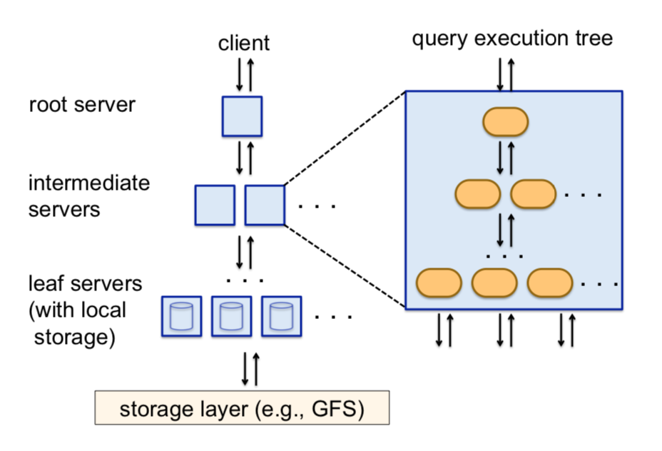
The crucial process in this serving tree is that of query-rewriting. How are queries rewritten? Fundamentally, a server at one level in the serving tree will rewrite its query such that the work the query does can be divided among the servers below it. Once the servers below get their results, the original server aggregates these results and passes it further up the serving tree. This repeats all the way to the root server. Classic divide-and-conquer.
Let’s look at an example. A root server may receive the following query from a client:
SELECT COUNT(A) FROM T
This query does a count of all A fields in the table T. It can be rewritten
into
SELECT SUM(C) FROM (R_1 UNION ALL ... R_n)
where R_i is defined as
SELECT COUNT(A) AS C FROM T_i
Here, T_i is a disjoint partition of the original table T. At the leaf
servers, such a partition is called a tablet. Each level of the serving tree
performs a further such rewrite of the query until the query reaches the leaf
servers. The leaf servers then scan their partition of T to do the actual
counting work. These counts are passed back up to intermediate serves, which sum
these counts into their own local count. At the root server, this sum becomes
the total count we originally wanted.
The end result of this recursive decomposition of the original query into smaller and smaller queries is that the final amount of work to be done by leaf servers is small in comparison to the overall work. This allows the entire query to be executed faster than if the root server had to scan the entire table sequentially itself. One experiment in the paper actually shows that changing the serving tree topology from 1:2900 (one root server, 2900 leaf servers) to 1:100:2900 (one root server, 100 intermediate servers, 2900 leaf servers) results in an order of magnitude performance gain for particular queries.
Query Dispatch
Finally, the paper touches upon interesting details about how Dremel approaches query dispatch. Specifically, this topic touches upon how Dremel deals with concurrent execution of multiple queries.
The paper explains that Dremel is, of course, a multi-user system, where many users can schedule queries at the same time. Dremel’s query dispatcher is responsible for coordinating the execution of these queries. This dispatcher has a notion of different levels of priority between queries, where higher priority queries are (probably) executed sooner than lower priority ones during times of high load.
To allow queries to execute in parallel, Dremel divides its capacity into
so-called slots. A slot is equal to one thread on a leaf server. For example,
a system with 3,000 leaf servers, each running 8 threads that could scan the
storage layer, has 3,000 x 8 = 24,000 available slots in total. Recall that a
table is itself partitioned into tablets. A single slot is assigned one or
more tablets that it alone can read from. If a tablet is split into 100K tablets, that means that each slot would be responsible for 5 tablets, of which it can read one at a time. If two queries need to access the same tablet, the slot would presumably be able to service only one of these queries and this is where a delay could occur for the second query.
For fault tolerance, each tablet is two to three-way replicated, such that if a
slot cannot reach a tablet, it can contact at least one other source of that
same tablet data. On the topic of tablets: It is unclear to me whether a tablet
can contain multiple columns, but I simplistically think of them as fixed-size
splits of one column. For example, one tablet may contain 50MB worth of data for
the Name.Language.Code field. The paper lists 100K-800K as typical examples
for the number of tablets for one table.
One very interesting mention in the paper is that the query dispatcher has a parameter that controls the percentage of tablets that must be read before a query is considered copmlete. It turns out that reducing this parameter from 100% to something slightly lower, like 98%, can result in “signficant” speedups to the overall execution.
Takeaways

Well, there it is: Dremel, a platform for “Interactive Analysis of Web-Scale Datasets”. What can we take away from it? I would say:
- Scan-based queries of read-only nested data can be executed at interactive speeds (<10s),
- Columnar storage can be applied to nested data just as it has been applied to relational data in DBMS,
- If trading speed against accuracy is acceptable, a query can be terminated much earlier and yet see most of the data.
Overall, I found the paper very well written and insightful on many fronts. I hope this article provided some further detail where more detail might have been necessary but was outside the scope of an academic paper. As such, query on!